
Drizzle is a technique for combining multiple exposures of the same scene that can recover resolution lost to undersampling. That’s the theory, anyway, and it does do what is says on the tin, but there is a problem: the recovered information usually has very low contrast. Comparing drizzled vs. non-drizzled images, it can often be hard to see any benefit, and one wonders whether it is worth the effort.
To see why this is, let’s look at the modulation transfer function plots for a typical setup: a Takahashi FSQ-106 with a QHY600M, based on the Sony IMX455 CMOS sensor with 3.76µ pixels.
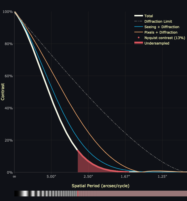
As can be seen, the maximum resolution that can be captured by this setup occurs at a spatial period of about 2.9 arcseconds/cycle, where the red shaded area begins. This is due to the pixels being too large to capture the resolution that the optics produce, resulting in undersampling. Details at scales that are finer than this – those within the red shaded area – are lost.
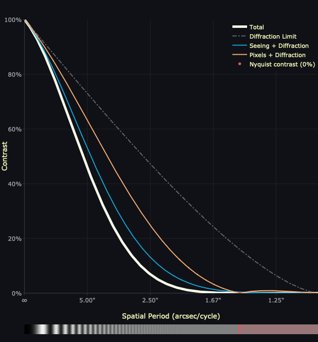
Performing drizzle combination of the original exposures with 2x upsampling results in the following MTF plot, identical to the first except that the Nyquist sampling frequency – where the red area starts – moves to twice the spatial frequency, or half the spatial period.
Drizzle does indeed recover this resolution, but the restored detail has low contrast. This is indicated by the low value of the white curve – the overall MTF of the system considering diffraction, seeing, and pixel convolution – in the recovered area. The contrast in this area starts at about 12.4% at the original Nyquist frequency, and tapers off toward zero from there. The low contrast can also be seen in the test pattern below the plot. What should be distinct full-black and full-white pairs of lines are instead washed out to a muddy grey.
Ideal deconvolution, where the point spread function (PSF) of the system is perfectly known, and where there is no noise in the image, should be able to recover this lost contrast. It will not only reverse the effects of seeing and pixel convolution, but also exceed the diffraction limit of the optics, represented by the dashed grey curve in the MTF plots. This is contrast lost due to the wave nature of light itself, inherent in all optical designs. The only way to change this in the image acquisition process is to use a telescope with a larger aperture – because of diffraction, even “perfect” optics are not perfect.
Deconvolution restores contrast regardless of what caused its loss. A truly ideal MTF plot would be a straight line across the top of the plot – 100% contrast at all spatial frequencies.
How close to this ideal can a real deconvolution algorithm come when run on a real image with noise and a real PSF? Can it recover the contrast in the area restored by drizzle combination? The theory says it can, but let’s put it to a practical test.
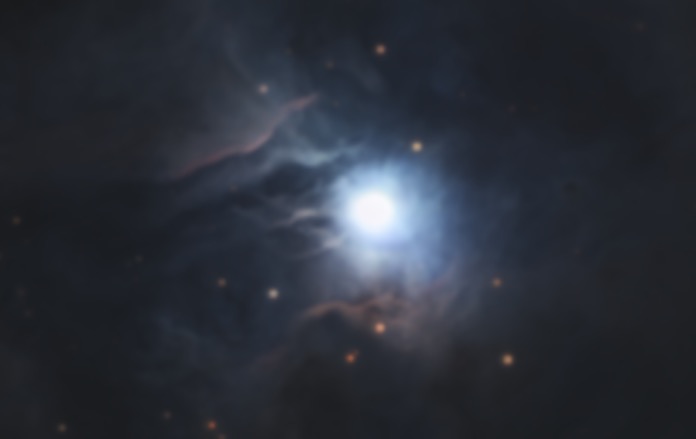
Here is a long integration of exposures of the Iris Nebula taken with the above setup. I’ve zoomed in on just the central part of the Iris – the full frame covers a much wider area.
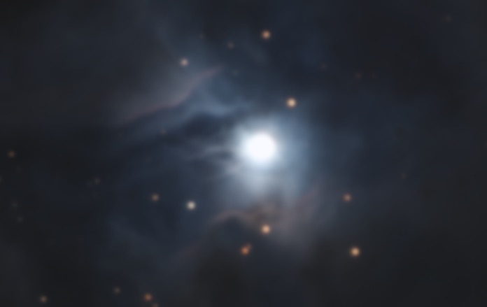
Here is the result when combining these same exposures with 2x drizzle combination:
It’s really not very impressive. Yes, the stars are a bit tighter, and there are some hints of additional detail in the delicate tendrils of the nebula surrounding SAO 19158, the bright central star.
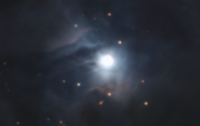
The theory says that drizzle should have recovered more than we can easily see at first glance, and the additional low-contrast detail should be able to have its contrast restored through deconvolution. To do a fair comparison, we need to first deconvolve the 1x image. Here it is again, but after applying BlurXTerminator:
And finally, here is the 2x drizzled image after applying BlurXTerminator with identical settings, save for the nonstellar PSF diameter, which was increased by 2x to account for the upsampling:
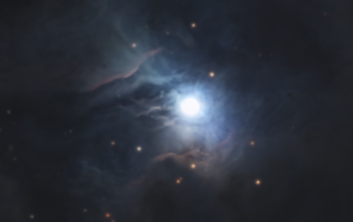
As can be easily seen comparing the last two photographs, 2x drizzle plus deconvolution really shines. Fine detail not resolved in the 1x image, and only hinted at in the 2x image without deconvolution, is now clearly visible. The theory works in practice, and the extra time, effort, and storage space consumed performing upsampled drizzle combination becomes worth the while.
Real deconvolution, run on real images, will always be fundamentally limited by noise. Noise represents a “floor,” as it were, in the MTF plots – a lower limit below which contrast cannot be recovered. To truly reap the benefits of drizzle plus deconvolution, the areas of interest should have very low noise, achieved by taking more and/or longer exposures. These exposures should also be well dithered – offset slightly from exposure to exposure – otherwise drizzle upsampling won’t have the information it needs from “between the pixels” to recover the lost fine detail.